Problem Description

Let G=(V,E) be an undirected complete graph, where V is the set of n vertices and E the set of edges. Each edge (u, v) ∈ E with u, v ∈ V has an associated distance d_uv between u and v. Dispersion, or diversity, problems (DP) consist in finding a subset S ⊆ V with m elements, such that an objective function (based on the distances between elements in S) is maximized or minimized. In this paper we focus on the Minimum Differential Dispersion Problem (Min-Diff DP). The Min-Diff DP is strongly NP-hard, and it remains NP-hard even if sign restrictions for distances between vertices are imposed (Prokopyev et al., 2009). Therefore, heuristic procedures emerges as the best option to obtain high quality solutions in shorter computing time.

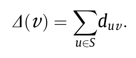
A feasible solution of the Min-Diff problem is a set S ⊆ V of m elements, where m is a given input parameter. Each feasible solution has associated with it a cost which can be computed as follows. Let Δ(v) be the sum of distances between a vertex v ∈ S and the remaining elements of S. Formally,

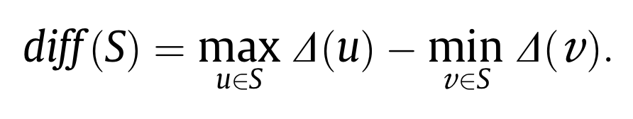
The objective function of a solution S, denoted by diff(S), is then computed as

Therefore, the Min-Diff problem consists of finding a solution S^★ ⊆ V with the minimum differential dispersion, i.e.

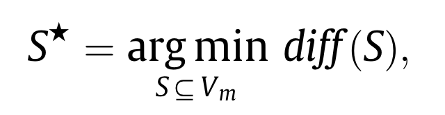
where V_m is the set of all subsets of vertices in V with cardinality m.

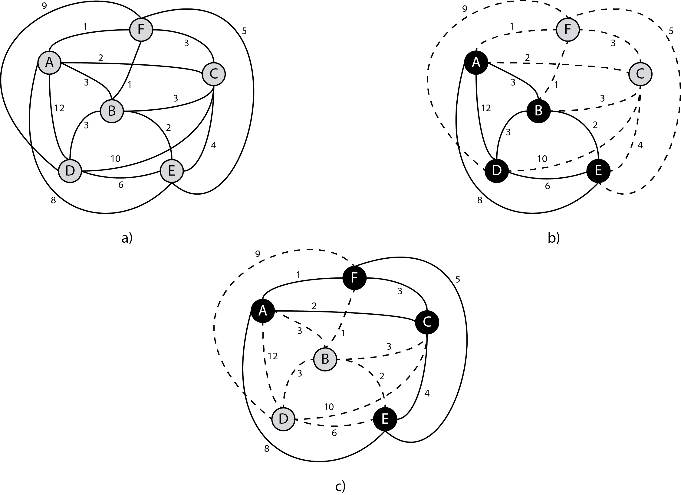
Figure 1.a shows an example of a graph with six vertices and 15 edges with their associated distances. Figures 1.b and 1.c depict two possible solutions for the Min-Diff problem for m=4. The selected vertices in the solution are shown in black while the edges in each solution are highlighted by solid lines. The vertices not in the solution are shown in grey while the edges not in the solution are dashed. To evaluate the quality of each solution, we first compute the Δ(v) value for all the elements in the solution. In particular, Figure 1.b shows a solution where S = {A, B, D, E}, Δ(A) = 3 + 12 + 8 = 23, Δ(B) = 3 + 3 + 2 = 8, Δ(D) = 12 + 3 + 6 = 21, and Δ(E) = 8 + 2 + 6 = 16. The diff-value is calculated by first selecting the vertices having the highest and lowest Δ-values and then taking the difference of their Δ-values. In this solution, these vertices are, respectively, A and B, and therefore diff(S) = Δ(A) - Δ(B) = 23 - 8 = 15 . If we now consider the solution S' = {A, C, E, F} in Figure 1.c, it is easy to verify that the associated objective function value is diff(S')= 9. Considering that the Min-Diff problem is a minimization problem, solution S' is better than solution S. The rationale behind this is that the distances among the elements in S' are more similar than those among the elements in S.

State of the Art Methods

The best algorithm in the state of the art is a GRASP method presented in Duarte et al. (2014). They propose two constructive procedures for the Min-Diff DP. The first one, C1, is based on a classical greedy-random strategy, while the second one, C2, inverts the greedy and random stages as introduced in Resende and Werneck (2004).

Authors also presents three local search methods which use an efficient evaluation of the objective function. The first local search, LS1, follows a best improvement strategy, while the second one, LS2, is based on a first improvement strategy. The last local search follows a first improvement strategy but the vertices to be moved are sorted according to their contribution to the solution.

The constructive and local search methods proposed are embedded in a variable neighborhood search algorithm. Specifically, authors propose a Basic VNS scheme where the classical neighborhood change is replaced by a jump neighborhood change method. Finally, the authors use two path relinking strategies to combine the solutions produced by the Basic VNS algorithm. The two variants are interior path relinking and exterior path relinking.

Instances

The set of instances used is the MDPLIB, which is divided into three sets:

1. SOM: This data set consists of 20 inter-node distance matrices of sizes ranging from n = 25 and m = 2 to n = 500 and m = 200. They have been used in most of the previous papers dealing with the maximum diversity problem.
2. GKD: This data set consists of 70 inter-node distance matrices for which distance values were calculated as the Euclidean distance between pairs of randomly generated points with coordinates in the [0,10] x [0,10] square. The sizes of these instances range from n = 10 and m = 2 to n = 500 and m = 50.
3. MDG: This data set consists of 100 inter-node distance matrices with real numbers randomly selected between 0 and 10 from a uniform distribution and size varying from n = 500 and m = 50 to n = 3000 and m = 600.

You can download the instances here.

Computational Experience

We performed extensive computational experiments the previously described instances. The best values found for each instance can be downloaded here.

References

- Duarte A., Sánchez-Oro J., Resende M.G.C., Glover F., Martí R. Greedy randomized search procedure with exterior path relinking for differential dispersion minimization. Information Sciences, in press (2014)
- Resende M.G.C., Werneck R.F.A hybrid heuristic for the p-median problemJournal of Heuristics, 10(1):59--88 (2004)