Quadratic Minimum Spanning Tree Problem
Problem Description
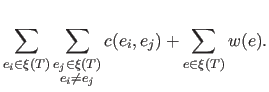
The Quadratic Minimum Spanning Tree Problem (QMSTP) may be defined as follows. Let G = (V, E) be an undirected graph where V={v1, ..., vn} is the vertex set and E={e1, ..., em} is the edge set. Consider that each edge and each pair of edges has an associated cost. In mathematical terms, we have two cost functions: w : E → ℜ+ and c : (E x E) - {(e, e), ∀e ∈ E} → ℜ+. We assume that c(ei, ej) = c(ej, ei) for i, j = 1, ..., m. The QMSTP consists of finding a spanning tree T of G with edge set ξ(T) ⊆ E that minimizes:
The QMSTP is an extension of the well-known minimum spanning tree problem, where in addition to edge costs, we have costs associated with pairs of edges. The problem was first introduced by Assad and Xu (1992), who showed that it is NP-hard and, since then, has been widely studied in the literature due to its applications in a wide variety of settings, including transportation, telecommunication, irrigation, and energy distribution.
State of the Art Methods
The most relevant metaheuristics developed to solve this problem are:
- GA: A genetic algorithm approach that employs an edge-window-decoder encoding. Soak et al. (2006).
- ABC: An artificial bee colony method combined with a local search procedure. Sundar et al. (2010)
- ITS: Iterated tabu search that alternates tabu search with perturbation procedures. Palubeckis et al. (2010).
- LS-TT: A local search algorithm with tabu thresholding. Öncan and Punnen (2010).
- TS-SO: A tabu search method that incorporates strategic oscillation by alternating between constructive and destructive phases. Lozano et al. (2013).
- IG: An iterated greedy algorithm with a local search phase for improving the reconstructed solutions. Lozano et al. (2013).
- HSII: It is a relay collaborative hybrid metaheuristic that executes TS-SO, IG, and ITS in a pipeline fashion. Lozano et al. (2013).
Instances
We considered three groups of benchmark instances for our experiments (in total constituting 83 instances), which are described below and available to download from here.
- The first set of benchmarks, henceforth denoted by CP, is composed of 36 instances, ranging in size from 40 to 50 vertices, and was introduced by Cordone and Passeri
- Öncan and Punnen present a transformation scheme to obtain QMSTP instances from quadratic assignment problem (QAP) instances. They demonstrated that the optimum value of a QMSTP instance obtained with this transformation is equal to the optimum value of the corresponding QAP instance. Particularly, the authors offered two instance sets by transforming 15 QAP instances (from n = 24 to 60) by Nugent et al. (1968) and 14 QAP instances (from n = 24 to 50) by Christofides and Benavent (1989) (whose optimal solutions are known). They will be denoted by NUG and CHR, respectively.
- The last group consists of two sets of large instances: RAND and SOAK. They were generated exactly in the same manner as in Zhou and Gen (1998) and Soak et al. (2006), respectively. All the instances in the RAND set represent complete graphs with integer edge costs uniformly distributed in [1, 100]. The costs between edges are also integers and uniformly distributed in [1, 20]. In the SOAK instances, nodes are distributed uniformly at random on a 500 x 500 grid. The edge costs are the integer Euclidean distance between these points. The costs between edges are uniformly distributed between [1, 20]. For each value of n ∈ {150, 200, 250}, there are 3 instances, leading to a total of 9 instances for each set.
Computational Experiment
We have performed a computational comparison of state of the art methods on the set of instances described above. All methods were stopped using the same time limit, which varied according to problem type and size, as specified in Table 1.
| Instance Type | Size | Time (seconds) |
|---|---|---|
| CP | All | 1 |
| NUG and CHR | All | 1000 |
| RAND and SOAK | 150 | 400 |
| 200 | 1200 | |
| 250 | 2000 |
Tables 2-5 show the results for state-of-the-art algorithms on different set of instances. For each algorithm, in column Avg-Dev, we include the average of the relative deviations from the best value known of the solution values found by the algorithm in the 10 runs on a set of problem instances and, in the case of the column %best, we outline the percentage of runs in which the algorithm reached the best value known for the instances in the corresponding group.
In addition, non-parametric tests have been used to compare the results of the different optimization algorithms under consideration. In order to detect the differences among pairs of algorithms, we have applied Wilcoxon’s test. Column Diff.? indicates whether Wilcoxon’s test found statistical differences between algorithms compared.
The experiments were conducted on a computer with a 3.2 GHz Intel© Core™ i7 processor with 12 GB of RAM running Fedora™ Linux V15
| Set | IG | SO | ITS | HSII | ||||
| Avg-Dev | %best | Avg-Dev | %best | Avg-Dev | %best | Avg-Dev | %best | NUG | 0.0745 | 0 | 0.0429 | 7.33 | 0.0104 | 15.33 | 0.0176 | 8.67 |
|---|---|---|---|---|---|---|---|---|
| CHR | 0.2434 | 10 | 0.0945 | 23.57 | 0.9918 | 10 | 0.0665 | 20 |
| RAND | 0.0016 | 8.89 | 0.0048 | 0 | 0.0046 | 0 | 0.0021 | 1.11 |
| SOAK | 0.001 | 6.67 | 0.0072 | 0 | 0.0016 | 3.33 | 0.0012 | 2.22 |
| CP | 0.0005 | 71.94 | 0.004 | 25.56 | 0.0004 | 77.50 | 0.0006 | 72.22 |
| Avg. | 0.064 | 19.5 | 0.031 | 11.292 | 0.202 | 21.232 | 0.018 | 20.844 |
| CP set | Wicoxon's test (HSII vs) | ||||
| Algorithm | Avg-Dev | %best | R+ | R- | Diff? |
|---|---|---|---|---|---|
| IG | 0.0005 | 71.94 | 300.0 | 366.0 | no |
| SO | 0.0040 | 25.56 | 664.5 | 1.5 | yes |
| ITS | 0.0004 | 77.50 | 182.5 | 483.5 | yes |
| ABC | 0.0061 | 20.28 | 661.0 | 5.0 | yes |
| HSII | 0.0006 | 72.22 | |||
| NUG set | CHR set | Wicoxon's test (HSII vs) | |||||
| Algor. | Avg-Dev | %best | Avg-Dev | %best | R+ | R- | Diff? |
|---|---|---|---|---|---|---|---|
| IG | 0.0745 | 0 | 0.2459 | 10.00 | 434.0 | 1.0 | yes |
| SO | 0.0429 | 7.33 | 0.0965 | 22.86 | 294.5 | 140.5 | no |
| ITS | 0.0104 | 15.33 | 0.9965 | 10.00 | 207.0 | 228.0 | no |
| ABC | 0.2597 | 0.00 | 1.9261 | 0.00 | 435.0 | 0.0 | yes |
| LS-TT | 0.0671 | 0.00 | 0.2918 | 7.14 | 411.0 | 24.0 | yes |
| HSII | 0.0176 | 8.67 | 0.0686 | 20.00 | |||
| RAND set | SOAK set | Wicoxon's test (HSII vs) | |||||
| Algor. | Avg-Dev | %best | Avg-Dev | %best | R+ | R- | Diff? |
|---|---|---|---|---|---|---|---|
| IG | 0.0016 | 8.89 | 0.0010 | 6.67 | 23.0 | 148.0 | yes |
| SO | 0.0048 | 0 | 0.0072 | 0 | 171.0 | 0.0 | yes |
| ITS | 0.0046 | 0 | 0.0016 | 3.33 | 162.0 | 9.0 | yes |
| ABC | 0.0111 | 0.00 | 0.0077 | 0.00 | 171.0 | 0.0 | yes |
| HSII | 0.0021 | 1.11 | 0.0012 | 2.22 | |||
References
- Assad A. and Xu W. (1992) The quadratic minimum spanning tree problem. Naval Re- search Logistics, 39(3), 399-417.
- Christofides N. and Benavent E. (1989) An exact algorithm for the quadratic assignment problem. Operations Research, 37(5), 760-8.
- Lozano M., Glover F., García-Martinez C., Rodríguez F.J. and Martí R. (2013) Tabu Search with SO for the Quadratic Mininum Spanning Tree. IIE Transactions, In press.
- Nugent C.E., Vollman T.E., and Ruml J. (1968) An experimental comparison of techniques for the assignment of facilities to locations. Operations Research, 16(1), 150-73.
- Öncan T. and Punnen A.P. (2010) The quadratic minimum spanning tree problem: a lower bounding procedure and an efficient search algorithm. Computers and Operations Research, 37(10), 1762-1773.
- Palubeckis G., Rubliauskas D., and Targamadz A. (2010) Metaheuristic approaches for the quadratic minimum spanning tree problem. Information Technology and Control, 39(4), 257-268.
- R. Cordone and G. Passeri, Solving the Quadratic Minimum Spanning Tree Problem, Applied Mathematics and Computation 218 (23), Pages 11597–11612, August 2012. http://homes.di.unimi.it/~cordone/research/qmst.html
- Soak S.M., Corne D.W., and Ahn B.H. (2006) The edge-window-decoder representation for tree-based problems. IEEE Transactions on Evolutionary Computation, 10(2), 124-144.
- Sundar S. and Singh A. (2010) A swarm intelligence approach to the quadratic minimum spanning tree problem. Information Sciences, 180(17), 3182-3191.
- Zhou G. and Gen M. (1998) An effective genetic algorithm approach to the quadratic minimum spanning tree problem. Computers and Operations Research, 25(3), 229-237.