Vertex Separation Problem
Duarte A., F. Escudero L., Martí R., Mladenovic N., Pantrigo J.J. and Sánchez-Oro J. (2012)
Optsicom project, University of Valencia (Spain)
Problem Description
Let G(V,E) be an undirected graph where V (n = |V|) and E (m = |E|) are the sets of vertices and edges, respectively. A linear layout φ of the vertices of G is a bijection or mapping φ : V → {1, 2, . . . , n} in which each vertex receives a unique and different integer between 1 and n. For vertex u, let φ(u) denote its position or label in layout φ. Let L(p,φ,G) be the set of vertices in V with a position in the layout φ lower than or equal to position p. Symmetrically, let R(p,φ,G) be the set of vertices with a position in the layout φ larger than position p. In mathematical terms,

Since layouts are usually represented in a straight line, where the vertex in position 1 comes first, L(p,φ,G) can be simply called the set of left vertices with respect to position p and, R(p,φ,G) the set of the right vertices w.r.t. p.
The Cut-value at position p of layout φ, Cut(p,φ,G), is defined as the number of vertices in L(p,φ,G) with one or more adjacent vertices in R(p,φ,G), then,

where N(u) = {v ∈ V : (u, v) ∈ E}. The Vertex Separation value (VS) of layout φ is the maximum of the Cut-value among all positions in layout φ: VS(φ,G) = maxp Cut(p,φ,G).
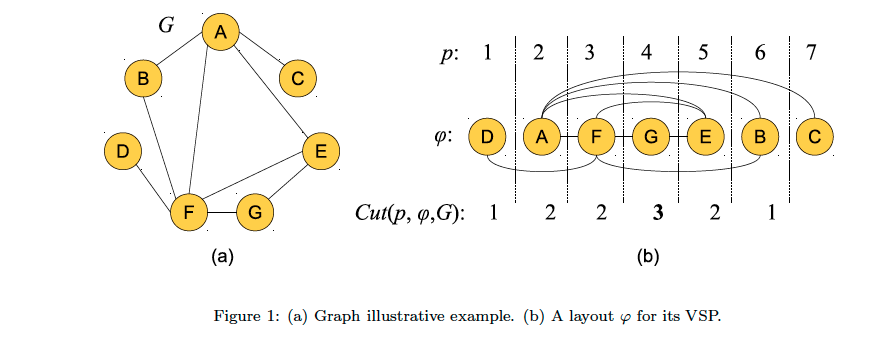
Figure 1.a shows an illustrative example of an undirected graph G with 7 vertices and 9 edges. Figure 1.b depicts a solution (layout) φ of this graph and the Cut-value of each position p, Cut(p,φ,G). For example, Cut(1,φ,G) = 1 because L(1,φ,G) = {D} and R(1,φ,G) = {A, F, G, E, B, C} and there is one vertex in L having an adjacent vertex in R. Similarly, Cut(3,φ,G) = 2 where L(3,φ,G) = {D, A, F} and R(3,φ,G) = {G, E, B, C}. The objective function value, computed as the maximum of these cut values, is VS(G,φ) = 3 whose related position is p = 4.
State of the Art Methods
The decisional version of the VSP was proved to be NP-complete for general graphs (Lengauer, 1981). It is also known that the problem remains NP-complete for planar graphs with maximum degree of three (Monien and Sudborough, 1988), as well as for chordal graphs (Gustedt, 1993), bipartite graphs (Goldberg et al. 1995), grid graphs and unit disk graphs (Diaz et al. 2001).
We can find many different graph problems that, although stated in different terms, are equivalent to the VSP in the sense that a solution to one problem provides a solution to the other one. Some of them are the Path-Width problem (Kinnersley 1992), the Interval Thickness problem (Kirousis and Papadimitriou 1985), the Node Search Number (Kirousis and Papadimitriou 1986} and the Gate Matrix Layout (Kinnersley and Langston 1994). The equivalence between these problems is a consequence of the results presented in (Fellows and Langston, 1994, Kinnersley 1992 and Kirousis and Papadimitriou 1986). For any graph G let VS(G), PW(G), IT(G), SN(G) and GML(G) be the objective function value of the optimal solution for the Vertex Separation, Path-Width, Interval Thickness, Node Search Number and Gate Matrix Layout problems, respectively. These values verify the following relations:
VS(G) = PW(G) = IT(G) = SN(G) - 1 = GML(G) + 1.
The VSP appears in the context of finding “good separators” for graphs (Lipton and Tarjan 1979) where a separator is a set of vertices or edges whose removal separates the graph into disconnected subgraphs. This optimization problem has applications in VLSI design for partitioning circuits into smaller subsystems, with a small number of components on the boundary between the subsystems (Leiserson, 1980). The decisional version of the VSP consists of finding a vertex separation value larger than a given threshold. It has applications on computer language compiler design and exponential algorithms. In compiler design, the code to be compiled can be represented as a directed acyclic graph (DAG) where the vertices represent the input values to the code as well as the values computed by the operations within the code. An edge from node u to node v in this DAG represents the fact that value u is one of the inputs to operation v. A topological ordering of the vertices of this DAG represents a valid reordering of the code, and the number of registers needed to evaluate the code in a given ordering is precisely the vertex separation number of the ordering (Bodlaender et al., 1998). The decisional version of VSP has also applications in graph theory (Fomin and Hie, 2006). Specifically, if a graph has a vertex separation value, say w, then it is possible to find the maximum independent set of G in time O(2w n). Other practical applications include Graph Drawing and Natural Language Processing (Dujmovic et al., 2008, Miller, 1956).
Instances (VSPLIB)
We have experimented with three sets of instances, totalizing 173 instances:
- HB: We derived 73 instances from the Harwell-Boeing Sparse Matrix Collection. This collection consists of a set of standard test matrices M = Muv arising from problems in linear systems, least squares, and eigenvalue calculations from a wide variety of scientific and engineering disciplines. The graphs are derived from these matrices by considering an edge (u, v) for every element Muv = 0. From the original set we have selected the 73 graphs with n ≤ 1000. The number of vertices and edges range from 24 to 960 and from 34 to 3721, respectively.
- Grids: This set consists of 50 matrices constructed as the Cartesian product of two paths (Raspaud et al., 2009). They are also called two dimensional meshes and the optimal solution of the VSP for squared grids is known by construction, see [7]. Specifically, the vertex separation value of a square grid of size λ × λ is λ. For this set, the vertices are arranged on a square grid with a dimension λ × λ for 5 ≤ λ ≤ 54. The number of vertices and edges range from 5 × 5 = 25 to 54 × 54 = 2916 and from 40 to 5724, respectively.
- Trees: Let T(λ) be set of trees with minimum number of nodes and vertex separation equal to λ. As it is stated in Ellis et al. (1994), there is just one tree in T(1), namely the tree with a single edge, and another one in T(2), the tree constructed with a new node acting as root of three subtrees that belong to T(1). In general, to construct a tree with vertex separation λ + 1 it is necessary to select any three members from T(λ) and link any one node from each of these to a new node acting as the root of the new tree. The number of nodes, n(λ), of a tree in T(λ) can be obtained using the recurrence relation n(λ) = 3n(λ - 1 ) + 1 where and n(1) = 2 (see Ellis et al. (1994) for additional details). We consider 50 different trees: 15 trees in T(3), 15 trees in T(4) and 20 trees in T(5). The number of vertices and edges range from 22 to 202 and from 21 to 201, respectively.
The VSPLIB contains 173 instances:
Computational Experience
All the algorithms were implemented in Java SE 6 and the experiments were conducted on an Intel Core i7 2600 CPU (3.4 GHz) and 4 GB RAM. We have considered the VSPLIB instances described above. The individual results for each instance can be downloaded here in Excel format.
References
- Bodlaender HL, Gustedt J, Telle JA. Linear-time register allocation for a fixed number of registers. Proc. of teh Symposium on Discrete Algorithms, 1998; 574–583.
- Díaz J., Penrose M.D., Petit J., Serna M. Approximating layout problems on random geometric graphs. Algorithms 2001; 39(1):78–116.
- Dujmovic V, Fellows MR, Kitching M, Liotta G, Mccartin K, Nishimura N, Ragde P, Rosamond FA, Whitesides S, Wood DR. On the Parameterized Complexity of Layered Graph Drawing. Algorithmica 2008; 52(2):267–292.
- Ellis J.A., Sudborough I.H., Turner J.S.. The vertex separation and search number of a graph. Journal Information and Computation, 1994; 113:50–79.
- Fellows MR, Langston MA. On search, decision and the efficiency of polynomial-time algorithms. Journal of Computing Systems Sciences 1994; 49(3):769–779
- Fomin FV, Hie K. Pathwidth of cubic graphs and exact algorithms. Information Processing Letters 2006; 97:191–196.
- Goldberg P.W., Golumbic M.C., Kaplan H., Shamir R. Four strikes against physical mapping of DNA. Journal of Computing Biology 1995; 12(1):139–152.
- Gustedt J. On the pathwidth of chordal graphs. Discrete Applied Mathemastics 1993; 45(3):233–248.
- Kinnersley N.G. The vertex separation number of a graph equals its path-width. Information Processing Letters 1992; 42(6):345–50.
- Kinnersley NG, Langston MA. Obstruction set isolation for the gate matrix layout problem. Discrete Applied Mathematics 1994; 54(2-3):169–213.
- Kirousis M, Papadimitriou C.H. Interval graphs and searching. Discrete Mathematics 1985; 55(2):181–184.
- Kirousis M, Papadimitriou C.H. Searching and pebbling. Theory of Computation Sciences 1986; 47(2):205–218.
- Leiserson CE. Area-Efficient Graph Layouts (for VLSI). Proc. of IEEE Symposium on Foundations of Computer Science, 1980; 270–281.
- Lengauer T. Black-White Pebbles and Graph Separation. Acta Informatica 1981; 16:465–475.
- Lipton RJ, Tarjan RE. A separator theorem for planar graphs. SIAM Journal of Applied Mathematics 1979; 36:177–189.
- Miller GA. The Magical Number Seven, Plus or Minus Two. SIAM Journal of Applied Mathematics 1956; 13:81–97.
- Monien B., Sudborough I.H. Min Cut is NP-Complete for Edge Weighted Treees. Theory of Computatiuon Sciences 1988;58:209–229.
- Raspaud A., Schröder H., Sýkora O., Török L., and Vrt'o I. Antibandwidth and cyclic antibandwidth of meshes and hypercubes. Discrete Mathematics, 2009; 309:3541--3552.